Systematic Identification of Preferred Orbits for
Magnetospheric Missions:
2. The "Profile" Constellation
Goddard Space Flight Center, Greenbelt, MD 20771
Vol 50, No. 2, April-June 2002, p. 149-171
Modified by the author
|
AbstractUsing orbital criteria developed in part 1 of this study [Stern, [1]], a "Profile" constellation mission is developed for studying the Earth's magnetosphere. The basic "Profile" has 6 satellites in each of two close orbits with apogee 25 RE or 20 RE, (Earth radii, 1 RE = 6371 km), but it can be extended to a "Twin Profile" mission with two coplanar constellations (total of 24 s/c), covering the magnetosphere end-to-end and requiring only one launch. One constellation of 12 then has apogee at midnight (or at other times, dusk), the other at noon (or dawn), and the two exchange positions every 6 months. The small satellites (17 kg, 29 w) will measure magnetic fields, ion and electron energy spectra, and plasma bulk flows. They require a minimal Δv and can therefore be flung off in pairs from a spinning mother ship, assuring a scientifically desirable spin axis and other benefits. Simulation codes derive the week-by-week coverage of 10 magnetospheric regions by the 12 satellites, as well as the annual number of hours certain formations occur, e.g. 9+ satellites within 2 RE of the tail's neutral sheet. Of particular interest is the tight clustering of 6 to 12 satellites at r > 23E (for 25 RE apogee), enhancing (at various times) local coverage of the substorm reconnection region, low latitude boundary layer and bow shock. The article concludes with a list of 30 targeted scientific investigation, each with its appropriate formation. IntroductionThe first part of this article [Stern, [1], henceforth denoted as S-1) tried to develop a procedure for identifying, among elongated Earth orbits, those best suited for studying the Earth's magnetosphere, especially in coverage of the tail's plasma sheet, the site of much magnetospheric activity. As useful as such coverage is for single-spacecraft missions, it is even more important for missions of multiple spacecraft, because it then greatly increases the probability of a large number of spacecraft simultaneously covering an interesting region. This is the second part, the design of a constellation-class mission based on the ideas of S-1. The mission was named "Profile," because its original aim was to obtain a near-radial profile of the equatorial region of the magnetosphere. As the mission concept evolved [Stern, [2, 3, 4]], the various aspects considered in S-1 were recognized and incorporated, a process greatly helped by a simulation software for evaluating magnetospheric coverage. Several modifications increased the versatility of the mission, e.g. the "two group" configuration which gave "superclusters" at apogee, and were described in talks at meetings of the American Geophysical Union (AGU). Following this introduction, the article contains four main parts and a summary:
1. Evolution of the "Profile" Concept and Orbits.1.1 "Constellation" MissionsThis article develops a plan for a scientific mission studying the Earth's magnetosphere, the space region dominated by the Earth's magnetic field. That is where radiation belts are found, as well as processes responsible for magnetic storms and for the polar aurora. The region extends up to about 100,000 km in most directions, but more than 10 times as far in the long magnetospheric tail, on the side facing away from the Sun. the magnetosphere and its physical processes are described in more detail in S-1 and in articles cited there. In the initial decades of the space age, most magnetospheric research was conducted by single satellites, visiting various regions and measuring their magnetic fields, plasmas, flows, waves and variations. Around 1985, however, this process reached the stage of diminishing returns. Enough data were on hand to produce reasonable models of average structure, and to model the gross features and average behavior of transient phenomena such as magnetic storms, substorms, auroral currents and the effect of interplanetary disturbances. On the other hand, for extracting global patterns, simultaneous observations at many points were required (Stern, [2, 5]), which led to proposals for "constellation" missions of multiple satellites. Later a "constellation" mission became part of NASA's "Living with a Star" program of studying the Sun-Earth environment. How should such a constellation be configured? One proposed strategy has been to distribute satellites as evenly as possible, each providing a "pixel" of an image of the magnetosphere, or of a selected region in it. The problem is that even 100 satellites are too few for a clear 3-dimensional image. Furthermore, an even distribution may be wasteful, since some regions need denser coverage while others can do with less. And finally, because the relative positions of satellites shift constantly, space and time variations are imperfectly separated and much of the correlation study has to be statistical. "Profile" represents a different approach: instead of trying to cover all space in a somewhat random fashion, satellites are placed in an orderly, linear pattern. The initial concept (Fig. 1) called for 12 satellites in the same elongated orbit, providing a more or less radial profile of the magnetosphere (hence the name "Profile"). These would be small, low-cost "cheapsats" with low perigee and an apogee of 20 or 25 RE, (Earth radii, 1 RE= 6371 km) and would pass perigee one hour apart. While such coverage is essentially 1-dimensional, it is very stable, because each point of the orbit is occupied by some satellite at 12 times, one hour apart, giving a true time dependence. Furthermore, since the orbit is shared, the satellites will not drift apart in longitude. The radial variation may be the most important one in studying physical processes, e.g. in the propagation of substorms, shocks and compressions. By using one of the preferred orbits of S-1, a relatively small number of satellites can achieve an unusually good coverage, and data analysis is relatively straightforward. Other advantages concerning spin, calibration, data downloading, clustering at apogee, day-night coverage etc., will be discussed in what follows.
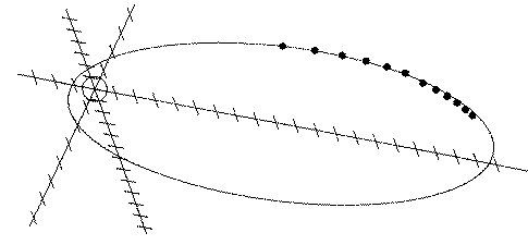
Figure 1. The original "linear" formation of "Profile": 12 s/c, 1 hour apart, 20RE apogee. 1.2 Distributing the Satellites along their OrbitThe original concept called for loading all satellites onto a "mother ship" in a near-equatorial orbit close to the desired one--e.g. perigee at radial distance rP = 1.1 RE (with a well-timed launch, rP later increases) and apogee of 20 or 25 RE (period 47 or 67 hours). At a selected perigee pass of the mother ship, a satellite is tossed ahead (or to the rear) with an extra velocity Δv that increases (or decreases) the orbital period by one hour. At the next perigee pass, the released satellite will lag behind the mother ship (or will lead it) by one hour, and then the next satellite is released in a similar fashion, and so on, every succeeding perigee pass. In the end all satellites occupy a new orbit, one hour apart. The mother ship could also be instrumented as a "baker's dozen" satellite, though its orbital period will differ by one hour. The satellites themselves are envisioned as low cost simple spacecraft, with no on-board propulsion and only simple sensors. Using state-of-the-art technology they could be constructed with a mass of 20 kg or less each. Typically, three types of data are of interest, all attainable with low weight and power consumption:
1.3 The value of ΔvA somewhat unexpected bonus of the release mode is the smallness of Δv. Let r1 be the radial distance at perigee, v1 the velocity there, a the semi-major axis of the orbit, T the orbital period and RE radius of the Earth, with all quantities expressed in meters or seconds. Then Kepler's 3rd law and the conservation of energy give From this Let a small change Δv in the perigee velocity produce a corresponding change ΔT. Then from the differential of (2), substituting (a/RE) from (1) But from (1) Because perigee distance is only slightly larger that RE, the first term is close to 2. The magnitude of the second term is less than 0.1, since the semimajor axis of these orbits is around 10.5 to 13 RE. Neglecting that term gives If ΔT = 1 hour, T = 48 hours, a = 10.5, v1 = 10370 m/s, we get With apogee around 25 RE, a similar calculation gives the speed of a slow runner. 1.34 The Centrifugal SlingshotTwo problems arise here. First, Δv for all satellites can vary at most by 0.5%, otherwise their periods will differ and their spacing will change. Secondly, the preferred spin axis is one perpendicular to the ecliptic, for two reasons. First, the plane of the plasma sheet tends to follow the ecliptic (apart from warps and shifts associated with the tilt of the dipole axis, as explained in S-1 ). The two velocity components which best describe bulk flows in the plasma sheet are therefore the ones in the plane of the ecliptic, and such a choice of the spin axis helps observing them. Secondly, if the satellite's solar cells are arranged around a cylinder (circular or polygonal), as they are in most spinning satellites, such an axis ensures a steady power level. But it is not easy to attain such spin: how can a satellite be given a Δv along its orbital path, if its spin axis is perpendicular to it, or steeply inclined? To impart Δv to a spinning spacecraft by a spring or a rocket, it must act along the spin axis. Here, to the contrary, the satellite needs a sideways toss, like a frisbee disk! A simple solution exists, however, if the mother ship has suitable attitude control. After it attains its elliptical orbit, it is turned until its axis is perpendicular to the ecliptic. It is then spun up (e.g. by a pair of small rockets), and the satellites swing out on extensible booms to a radius at which their linear velocity of rotation equals the required Δv. Each satellite is released at the required spin phase (determined by a sun sensor), to fly off tangentially forward or backwards with the required Δv. By conservation of angular momentum, it will continue spinning around the same axis with the same angular velocity as the mother ship. If the mother ship spins at 20 rpm and the radius of rotation--from the axis to the center of gravity of a satellite--is 1 meter, then the linear velocity will be 2.09 m/s, quite adequate for an apogee of 25 RE. The centrifugal acceleration (Δv)2/r will be about 4 m/sec2 or 0.4 g. At 40 rpm the velocity Δv doubles and the acceleration quadruples, still quite acceptable. Other radii and spin rates can be chosen to fit engineering considerations: as long as the radii of all arms are kept accurately equal, so will be the values of Δv.
There will however be one big departure from the original plan of Fig. 1. To prevent unbalancing of the mother ship, satellites will have to be released in opposite pairs. Rather than 12 satellites sharing the same orbit, the mission now has 6 in a higher orbit and a period one hour longer than that of the mother ship, and 6 in a lower orbit and a period shorter by one hour. If the spin axis is not exactly perpendicular to the orbital plane--e.g. a spin axis perpendicular to the ecliptic, and an orbital plane inclined at 13.5°, as in orbit #10 of S-1, cited further below--then the orbital inclinations of the two groups will also differ slightly.
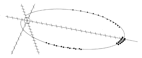
Figure 2 Three different formations with 2 groups of 6 s/c each, 1 hour apart, approx. 20RE apogee. 1.5 Missions with Two GroupsThe separation of satellites into two groups, with slightly different orbital periods, actually enhances the scientific capabilities of the mission. The two groups overtake each other (squares in Fig. 2) every T/2 orbits or T2/48 days--every 6.5 weeks for T=47 hrs, every 13.4 weeks for T=67 hrs. At those times the calibrations of their instruments can be accurately compared. Furthermore, as satellites approach each other while overtaking and then recede again, the 2-point correlation function of the magnetic field and of plasma properties can be observed. That function, important to the characterization of an isotropic turbulent plasma, can be compared simultaneously at each pair of overtaking satellites.. In either group, the spacing between neighboring satellites equals the distance they cover in one hour. Since speed greatly decreases towards apogee, the separation in kilometers is much smaller there, causing them to cluster there densely. When this happens during the time when satellite groups overtake each other, a "supercluster" develops (Fig. 2, dark circles), with 10 or more satellites in a radial distance spread of 2 RE (see part 3 of this article). On the other hand, near Earth the overlapping groups can give 24 consecutive traverses of the ring current within about 10 hours, along practically the same track, each satellite giving a 2 hour inbound traverse followed by an equal outbound one. Even though the observed ion spectrum (to 30 keV) falls short of the peak energies of the inner ring current (about 65 keV), such dense monitoring should help understand variations of the ring current and provide valuable information on convection in the inner magnetosphere and its dawn-dusk asymmetry. At other times the satellites will be spread linearly as in Fig. 1 (triangles in Fig. 2). At still other times the two groups will be on opposite sides of their orbital ellipses (formation not drawn) providing a measure of 2-dimensional coverage, in the sunward x-direction and the transverse y-direction (geocentric solar magnetospheric coordinates or GSM).
Figure 3. Schematic view of the "Twin Profile" mission, at the two times of the year when its satellites would explore the noon-midnight region. 1.6 The "Twin Profile" OptionThe axis of the orbital ellipse (line of apsides) shifts rather slowly in inertial space (due to non-Keplerian perturbations), and therefore as noted in S-1, it tends to rotate around the magnetosphere with a 1-year period. This occurs because the long axis of the magnetosphere is oriented by the flow of the solar wind, which approximately follows the Sun-Earth direction and therefore each year undergoes a 360° rotation in inertial space. An intriguing possibility is therefore to launch twin "Profile" missions into orbits that are mirror images of each other, sharing the same orbital plane but with apogees 180° apart. One mission might be launched from 10° north of the equator, with apogee at midnight during the northern summer solstice, while its "mirror image" would be launched from 10° south of the equator and its apogee at that time would be at noon (Fig. 3). Such a twin mission of 24 satellites could provide a complete radial profile, from the foreshock to the plasma sheet, every 6 months, with the satellite groups periodically exchanging roles. The two groups may also have different apogee distances, so that while one (for instance) has its densest plasma sheet coverage at 25E, the other would have it at 20 RE
Interestingly, both missions could also use a single vehicle launched from 10° north, or inserted into an orbit inclined 10° to the equator. The two mother ships would be stacked on top of each other, each with its own propulsion and its own attitude and spin-up control. A single rocket would place them in a circular parking orbit, where they would separate and would be pushed apart a short distance, enough for one to be fired without affecting the other. The upper stage rockets would then be fired eastward from two points on the parking orbit, 180° apart, points selected to place the orbital apogees at midnight at the two solstices (Fig. 3).
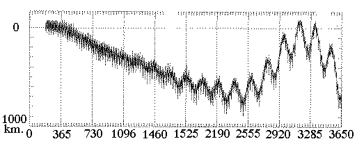
This scenario works well only if both orbits are "optimal" by the selection criteria of (S-1). If it were to turn out, for instance, that their semiannual perigee fluctuations were 180° out of phase, then using the same launch vehicle would require a delay in the firing of the upper stage of the second payload, not by half an orbit but by 3 months. Luckily, this does not happen and the semi-annual fluctuations of both perigees are initially exactly in phase. Fig. 4 shows the difference in perigee radius rP (km.) between orbit #10 of S-1 (apogee 25E) and its "matching twin" #10a, over a 10-year period. These orbits are discussed further below, and their coverage of the magnetosphere is later compared in Table 2. Even after 10 years, perigee values of the twin orbits are almost the same, though a small difference develops. The dense "noise" evident in the trace comes from the semi-monthly perigee variation, which clearly differs between the two orbits, but whose amplitude is rather small. The 10-year variations of the orbital elements of this "Twin Profile" mission were also compared and were found to be remarkably similar, except of course for a 180° shift of the argument of perigee. The date when apogee passes midnight advances about 12 days/year in both missions, so that apogees remain on opposite sides of Earth. The main change is in the duration of distant eclipses. Unfortunately, fine-tuning one set of 12 s/c to pass χ=0 when apogee is at noon [see S-1] ensures that the other is at that time at midnight, exposing it to eclipses of the greatest possible duration. Besides providing end-to-end coverage of the magnetosphere, the "Twin Profile" strategy has other benefits. Around equinox the two groups would be in a good position to compare dawn and dusk sectors of the magnetosphere and of its boundary layers, assessing asymmetries such as those associated with the By component of the interplanetary magnetic field. The coverage of the ring current at any time would be doubled. Also, no additional tracking stations would be needed to handle data downloading from the twin missions. Downloading is usually performed near perigee, typically requiring 4 stations approximately evenly scattered around the equator, assuring that at any perigee pass, at least one station would be in favorable position. Unfortunately, that results in a relatively low duty cycle, because while one station is kept busy, the one on the opposite side of Earth is necessarily idle. With the 24-satellite twin constellation, when one station is set to download from one of the groups, its counterpart on the opposite side is in a preferred position to download data from the other. This does not mean all stations share equally in the downloading task, for the times of perigee passage may differ, but it does suggest that the same stations can handle both sets with no interference. (2) Spacecraft Design
|

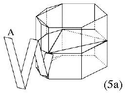
| Figures 5a-5c. Tentative design of a "Profile" satellite and its mother ship |
The design proposed here should be viewed as no more than a starting point, a "strawman design" only moderately changed from an earlier one [Stern, [3]]. By the original design, the frame of each satellite is a hexagonal cylinder (more strictly, prism), with sides 40 cm high and 25 cm wide. Outlining the hexagon, halfway between the top and bottom of the satellite, are three triangular shelves on which the instruments rest (Fig. 5a). The middle points of two shelves contain "strong points" by which the satellites are attached to the mother ship. A hinge at the juncture of two shelves is the attachment point of the folding boom which connects the satellite to the mother ship, and two other "strong points" are at the ends of the vertical members from the other ends of those shelves (see Figs. 5b and 5c). The top and bottom of the cylinders contain lighter framing and diagonal braces, which may hold insulating thermal blankets.
The folding boom may also hold the magnetometer. In that case, it must be non-magnetic, and as soon as it deploys, it should lock rigidly. When the satellite is let go, the separation will occur not at the boom's attachment to the body of the satellite, but just beyond the location of the magnetometer. The boom remaining with the satellite should be short enough to avoid hitting during release any other satellite still attached to the mother ship.
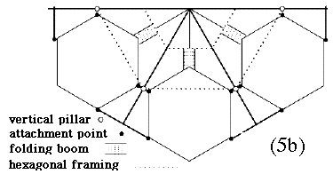
A smoother power output is obtained if the satellite has not 6 but 12 sides, each with a solar panel of GaAs cells; each shelf now has one stiff long side, and 4 equal short sides, each supporting a panel. For simplicity, only one shelf in Fig. 5a was drawn this way, while the other two were left in the original hexagonal configuration; the frames on top and bottom were also omitted. The attaching boom is also schematically drawn (slightly extended, for clarity), and A marks the end at which it is attached to the mother ship.
The mass of each satellite was estimated at 17 kg, including 4 kg for the frame and 4.7 kg for the solar panels, which include a glass cover 1 mm thick to reduce radiation damage from the inner radiation belt. The panels are estimated to generate 29 watts, including a 7-watt safety margin for the power loss due to accumulating radiation damage. Since the transmitter is expected to require 15 watts of power, it will not need any stored energy: mass is invested in a large solar array rather than in storage batteries. A small "keep alive" battery (0.5 kg) will keep the memory of 200 Mbits from losing data during passes in the Earth's shadow, as well as keeping it and the data processor warm during such times. Scientific instruments will be turned off during such passes, but "housekeeping" data monitoring temperatures and other aspects will be collected in the shadow and in the penumbral stages before and after the pass.
Other mass allocations are 3 kg for the transponder, 2 kg for scientific instruments, 1 kg for the module incorporating computer, memory, data handling and command (an estimate based on recent technology), 0.3 kg for sun-and-moon sensor, 0.5 kg for the antenna and preamplifier, and 1 kg for wiring. Since this article was first submitted (9.12.00), the planning of NASA's ST-5 "Nanosat Constellation Trailblazer" mission has addressed many of the problems of satellites in this mass range, and is later expected to launch small satellites that will test its design in actual space flight.
2.2 Data downloading
Data downloading is to be performed near perigee at a typical distance of 0.5 RE, and is based on conservative assumptions--an S-band transceiver and an omnidirectional antenna, possibly replaced by switchable antenna arrays or belt antennas. Data will be collected at 0.5-1 kb/s (depending on the mode) and by one strategy, data transmission to the ground will begin automatically at some distance (e.g. 2.5 RE radial) and will continue through the perigee pass, re-transmitting the data over and over again. Doppler information about the orbit would also be obtained. Data will be downloaded to 4 automatic stations distributed around the globe, e.g. New Mexico, Dakar, Oman and Brisbane, using 11-meter antennas. Currently such antennas cost about $750,000 each, and receiving stations about $500,000.
Earlier discussions of data downloading included many additional details [Stern, [3]], but these are omitted here because new technology may greatly improve the situation. The report of NASA's mission definition team for the "Draco" constellation mission proposes downloading an amount of data comparable to the one expected here (200 Mb), from a radial distance of about 3.5 RE, using an X-band transmitter of only 3 or 4.5 watts, with mass of just 0.15 kg. This data transmission is about 30-100 times faster than one extrapolated from the preceding estimates. If such a technology is available to "Profile", its data rate can rise considerably, while the mass of the spacecraft may drop below 15 kg. On the other hand, a more conventional design may be preferred, adding 3-4 kg of weight in storage batteries.
2.3 Eclipses and Radiation
Several technical problems remain to be solved. A nominal 2-year mission would include two seasons in the plasma sheet (4 seasons with "Twin Profile"), but since the mission is highly synergistic with any other mission to the magnetosphere, extending it seems an attractive option. Unfortunately (as described in S-1), it is difficult to avoid deep eclipses for much longer than two years, so that beyond the nominal mission, satellites may well encounter severe chilling near apogee.
Several possible remedies exist. Clustering sensitive electronics together reduces heat loss and creates some mutual shielding during passages of the inner radiation belt, and thermal blankets also help. To avoid overheating during normal operation (in particular when data are downloaded) the power stage of the transmitter may be mounted separately near the antenna, and that part of the system should be designed to withstand extreme chilling.
The element most sensitive to chilling is the battery. One possible solution is to make the operation of "Profile" satellites completely battery-free (at least as a contingency option), with the spacecraft "going to sleep" in the Earth's shadow and "reawakening" afterwards. Proposals of battery-free satellites have been made in the past, but no such mission was ever flown. It would require a non-volatile memory, a newly evolving technology requiring extra power for recording data--but as noted, except for times of data downloading near perigee (where no data are recorded anyway), ample power should be available. Thermal information then might not be collected in the deep shadow, but may still be available from partial eclipses and penumbral passes.
Radiation dosage from the inner belt has been estimated at 25 rad/pass (two passes per orbit), and with a 2-day orbit this adds up to about 10,000 rad/year. Most sensitive are the solar cells, which would need extra shielding by 1 mm glass, firmly bonded, and would even then gradually lose up to 25% of their power production. Space electronics exist that are rated to 100,000 rad, making the expected dosage tolerable.
2.4 Scientific Instruments
The scientific payload would contain (at the minimum) a 3-axis fluxgate magnetometer and a "top-hat" detector for ions and electrons covering the range 0.1-30 keV. Magnetometer technology is well developed and a state-of-the-art design (Goddard SFC proposal for "Rosetta") has 50 mg sensors with a resolution of 0.125 nT, power requirement 150 mW and mass of boom and electronics about 0.5 kg. Again, the ST5 mission is expected to provide actual tests of instruments like the ones proposed here.
A boom is needed put some distance between the magnetometers and the spacecraft circuitry, even if the latter is "magnetically clean." One strategy would place the instrument halfway down the folding boom which attaches each spacecraft to the mother ship (Fig. 5a) and to release the s/c by severing the boom just past that point.
An ion-electron detector in the style described by [Sablick et al., [6]] can be constructed with a mass of less than 1 kg and requiring just 1 watt, using techniques that tightly integrate the electronics with the analyzer. It can detect ions and electrons from 0.1 to 30 keV and is used as described in sect. 1.2.
Light rejection of such an instrument is good, which helps in observing the solar wind and magnetosheath. The high directional intensities in those regions, however, may saturate the detectors, and therefore an electrostatic deflector would be added internally and would turned on outside the magnetopause (also close to it on the inside, the region of the low latitude boundary layer), perhaps only in part of each spin cycle. It would defocus particles before they reach the detector, reduce sensitivity and prevent overloading. Well inside the magnetopause sensitivity could be kept high, so that bulk velocities can be derived by comparing ion spectra from two opposing directions.
2.5 The Mother Ship
The design of the mother ship, outlined below, is even more tentative than that of the satellites, and should only be regarded as the starting point of a more thorough engineering study. The design described here is essentially a cage holding the 12 satellites in two layers of 6 each, arrayed around a hexagonal girder 120 cm high, restraining the satellites during launch. Later on, as the mother ship spins, they will be held by long extensible booms, up to the moment when they are let go.

Fig. 5b views half of that configuration from above, while Fig. 5c gives its view from the side. The cage contains 4 sets of 6 radial struts each, connected by four hexagons with vertical separation of about 40 cm ("vertical," "top" etc. refer here to the orientation before launch). The struts and hexagons would be connected by 6 vertical struts and by a central pillar. The linked struts at the top and bottom of the cage, shorter than the other two sets, will also be connected by smaller hexagons. Each side of that hexagon will hold a hinge, anchoring one end (point A in Fig. 5a) of the folding boom connected to the nearest satellite.
Each boom will consist of 4-5 plates, about 5-7 cm wide, hinged to each other like pleats in a piece of material, and hinged at the satellite end to the junction of two of the shelves. A bolt or cable will link the attachment point to the central pillar, stopping the boom from deforming the side of the inner hexagon and thus changing the effective radius of rotation.
When the mother ship is spun up, the centrifugal force (helped by suitable springs) will pull the satellites out to the limits of the booms. The width of the hinged plates will resist sideways motion, which might cause collisions with other satellites in the same layer. The fact that the booms are anchored at the top and bottom of the cage (Fig. 5c) makes the two layers swing out away from each other, again reducing the chance of accidental contact. All this is of course only a preliminary "strawman" plan, almost certain to change.
Prior to the spin-up each satellite will be cradled by 4 strong points in the cage (Fig. 5c). The two inner points will be tied to the vertical struts and will support two of the central shelves of the satellite. The other two will be at the edges of the satellites, attached to the two middle sets of radial struts of the cage, in a way that the satellites naturally deploy away from their supports. The inner supporting struts used here will extend about 25 cm further than the outer ones (Fig. 5c) and braces will help support those extensions during launch, when they might have to resist accelerations of up to about 10g.
The middle layer of the cage will carry solar cells for use by the mother ship and instrumentation, as well as inertia wheels. Arms with spin-up rockets that swing out widely would also be attached there (not drawn). After the ship reaches its final orbit, it would separate from the last rocket stage, slowly turn around to the required direction, then the arms would swing out, the rockets would fire and the cage would be spun up. The restraints holding the satellites to the cage would be released and they would swing out and be ready for deployment.
The bottom of the cage would be a pallet able to support the entire structure during launch. If a "twin profile" is launched, the lower cage may need extra strength to support the weight and g-forces due to the upper one and again, all these details are open to revision.
In principle, one could dispense with spin-up rockets and instead have two cages, one per layer, able to rotate relative to each other. A large sprocket wheel would be attached to one, with a motor (or two) driving it by gears or by a cable wound around a drum. When the motor is started up, the assemblies start rotating in opposite directions, but since each releases its satellites in pairs, the final orbits are similar, except that 6 satellites now spin in one sense and 6 in the opposite one (in "Twin Profile" the two mother ships could be spun up instead). The two assemblies would separate before launch, and each would act as an independent "mother ship." Such an arrangement however might overcomplicate the mission, especially since the two spin rates must match exactly--or if different, their difference must be compensated by booms of different length.
2.6 The Draco Mission
A "magnetospheric constellation" is currently planned by NASA as part of its "Living with a Star" program (the star being the Sun). A mission definition team, appointed by NASA, has selected "DRACO" (Dynamics, Reconnection And Configuration Observatory), a 100-spacecraft mission for "Resolving Complex Plasma Dynamics in the Earth's Vast Magnetotail" [Note: This number has been revised a few times since publication]. A preliminary report has been issued, but it included no simulations of the type discussed further below.
The DRACO mission assumes orbits with perigee of 3 RE and apogees increasing in steps of 2 RE from 12 to 42 RE, or by another version, from 7 to 40 RE. In the original plan, each satellite was envisioned to have a mass of 10 kg (this may have been later increased), with instrumentation similar to the one proposed for "Profile," except for an additional solid-state telescope observing ions and electrons between 0.4 and 1 MeV. The design also calls for on-board propulsion. All this is considerably more than is proposed here for a 17 kg "Profile" spacecraft, but more advanced technology is envisioned. Whenever such technology becomes available, "Profile" plans could certainly benefit from it, too.
One great difference is the high perigee of the orbits. A high perigee has two advantages: it avoids the inner radiation belt, and it decreases the effect of the Earth's equatorial bulge. If low-perigee orbits were used and initially all orbits started from the same longitude, the bulge would cause them to separate fairly rapidly to different longitudes. Its great disadvantage is the greater distance for data downloading--typically 2.5 RE from the tracking station against 0.5-1 RE for a low perigee orbit, reducing signal intensity by a factor 6 to 25. In addition such orbits add to the space debris problem, whereas low-perigee orbits typically re-enter the atmosphere within a decade or two.
Comparison of scientific use is difficult, because no detailed simulation of "Draco" coverage of the magnetosphere has been described. Because "Draco" combines satellites of different periods and orbits, its formations would constantly change, so that rather than analyzing a well-ordered system, data analysis might have to fit models to observations by least squares or by a similar method. In addition, "Draco" lacks the concentrated observations by "superclusters"; also, to match the wider coverage of a "Twin Profile" mission, it too would have to double its number of its satellites. And the simultaneous tracking and data downloading of 100 satellites greatly exceeds that of any past mission: it might be safer to start with a more modest number of spacecraft.
Overall, the merits of these two different approaches deserve to be carefully compared before NASA decides on its initial "Constellation" mission.
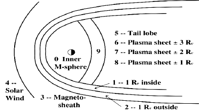
Figure 6 The classification of magnetospheric regions used in this study (from S-1)
3. Orbital Simulations
3.1 Science Goals
Space missions have a high cost in money, time and professional effort. Their scientific goals therefore need to be carefully chosen, and wherever possible, their observations and data analysis should be planned and simulated in advance. In geocentric solar magnetospheric (GSM) coordinates, the "Profile" orbit undergoes an annual rotation around the magnetosphere, and therefore each season brings different observations. When apogee is in the tail, "Profile" would observe substorms in various modes: "superclusters" at apogee may pin down the early stages, while "linear" formations would observe and measure the spread of waves, particles and of bulk motions which accompany and precede them. At still other times, with satellite groups at opposite flanks of the orbit, it could derive the lateral spread and expansion of substorms.
"Profile" would also study the quiet geotail, its 2-point correlations, its boundary layers, signatures of poleward arcs seen in the polar cap, bulk motions and reactions to dayside compressions. At both quiet and disturbed times, it would allow synergistic correlations with observations of NPOESS satellites in the polar cap, on the same field lines, with auroral images and with the state of the IMF. As noted earlier, the "Twin Profile" mission would make such dayside-plasma sheet correlations particularly extensive.
Later (and earlier) times will exist each year when apogee covers the low latitude boundary layer, allowing this layer to be observed by concentrated clusters (5-6) and by superclusters (up to 10, 11 or 12) of spacecraft. That region is particularly interesting because both plasmas on whose boundary it occurs--plasma sheet and magnetosheath--dominate their magnetic fields and are only moderately stiffened by magnetic field lines. The flaring angle can be monitored when the two groups of satellites are on opposite sides of their orbits, and waves and fluctuations of the boundary are then readily tracked.
On the dayside, waves, compressions and shocks are of interest, also plasmas in the sheath and foreshock, with occasional "superclustering" in interesting regions. Subsolar erosion and reconnection can be observed, and "Twin Profile" can relate them to simultaneous changes in the tail. In addition to all these, frequent passages of the ring current allow close tracking of changes associated with storms, substorms, compressions and IMF turnings.
Simulations help mission planners estimate ahead of time whether the formations which address each of these problems actually occur frequently enough. The method for doing so was already alluded to in S-1: track the satellites hour by hour (or more frequently) for one year, and analyze their positions. In S-1 only the simplest analysis was described--assigning each spacecraft to a region and finding for how many hours during the year each region is covered. In what follows below, this work is reviewed in more detail (Table 1), after which more detailed questions are posed and their results tallied (Table 3).
3.2 Coverage of Regions by single satellites
As described in S-1, locations (x,y,z) of the satellites (in GSM coordinates) were assigned, at hourly intervals throughout the year, to one of 10 regions, identified by region index IREG = 0, 1,... 9 (Fig. 6)
| IREG | Region | IREG | Region | |
| 0 | Inner magnetosphere | 5 | Tail lobe | |
| 1 | 0-1 RE inside magnetopause | 6 | Plasma sheet, 2 < |Δz| < 3 | |
| 2 | 0-1 RE outside magnetopause | 7 | Plasma sheet, 1 < |Δz|< 2 | |
| 3 | Magnetosheath | 8 | Plasma sheet, |Δz| < 1 | |
| 4 | Solar Wind | 9 | Transition region, 6 to 8 RE |
Table 1 gives week-by-week tallies for a selected orbit, the one numbered #10 in Table 3 of S-1 and also in the two tables further below. That orbit assumed eastward launch from northern latitude 10° on July 4, 2000, at the "reference time" when perigee had its most southward inclination to the ecliptic (13.5°). As described in a later note (June 2003), such orbits are also readily attainable from Cape Canaveral, given a modest Δv from a suitably timed additional mid-orbit firing. The table gives the average number of hours (rounded to an integer) accumulated daily by the 12 satellites in each value of IREG. They should add up to 288 (12 satellites, 24 hours) but the actual number fluctuates because of the averaging; the listed date is the 4th day of each week.
Table 1
| ||||||||||
| IREG= | 0 | 1 | 2 | 3 | 4 | 5 | 6 | 7 | 8 | 9 |
| Date | ||||||||||
| 6 7 00 | 23 | 0 | 0 | 0 | 0 | 79 | 50 | 72 | 64 | 0 |
| 13 7 00 | 28 | 0 | 0 | 0 | 0 | 58 | 57 | 73 | 71 | 0 |
| 20 7 00 | 24 | 0 | 0 | 0 | 0 | 75 | 44 | 58 | 86 | 0 |
| 27 7 00 | 27 | 0 | 0 | 0 | 0 | 68 | 44 | 68 | 81 | 0 |
| 3 8 00 | 25 | 6 | 0 | 0 | 0 | 50 | 62 | 79 | 65 | 0 |
| 10 8 00 | 21 | 77 | 0 | 0 | 0 | 41 | 41 | 50 | 52 | 0 |
| 17 8 00 | 19 | 67 | 72 | 2 | 0 | 18 | 37 | 29 | 36 | 4 |
| 24 8 00 | 21 | 37 | 56 | 80 | 0 | 13 | 20 | 25 | 28 | 4 |
| 31 8 00 | 23 | 27 | 35 | 121 | 0 | 27 | 20 | 11 | 16 | 4 |
| 7 9 00 | 24 | 20 | 23 | 170 | 0 | 2 | 11 | 9 | 19 | 5 |
| 14 9 00 | 35 | 19 | 22 | 162 | 0 | 12 | 12 | 6 | 15 | 4 |
| 21 9 00 | 28 | 16 | 14 | 185 | 21 | 9 | 7 | 1 | 6 | 0 |
| 28 9 00 | 39 | 15 | 18 | 112 | 74 | 6 | 9 | 3 | 10 | 0 |
| 5 10 00 | 26 | 9 | 10 | 74 | 152 | 6 | 6 | 2 | 2 | 0 |
| 12 10 00 | 39 | 13 | 12 | 75 | 128 | 6 | 8 | 2 | 5 | 0 |
| 19 10 00 | 26 | 8 | 10 | 45 | 188 | 3 | 5 | 1 | 2 | 0 |
| 26 10 00 | 37 | 12 | 10 | 48 | 166 | 2 | 7 | 2 | 4 | 0 |
| 2 11 00 | 26 | 8 | 9 | 36 | 200 | 0 | 2 | 3 | 2 | 3 |
| 9 11 00 | 31 | 9 | 9 | 31 | 191 | 0 | 0 | 4 | 2 | 10 |
| 16 11 00 | 31 | 8 | 9 | 28 | 205 | 0 | 0 | 0 | 0 | 6 |
| 23 11 00 | 37 | 8 | 8 | 26 | 207 | 0 | 0 | 0 | 0 | 2 |
| 30 11 00 | 44 | 9 | 9 | 24 | 203 | 0 | 0 | 0 | 0 | 0 |
| 7 12 00 | 33 | 8 | 8 | 20 | 220 | 0 | 0 | 0 | 0 | 0 |
| 14 12 00 | 46 | 10 | 10 | 22 | 199 | 0 | 0 | 0 | 0 | 0 |
| 21 12 00 | 31 | 7 | 7 | 14 | 229 | 0 | 0 | 0 | 0 | 0 |
| 28 12 00 | 46 | 10 | 10 | 25 | 196 | 0 | 0 | 0 | 0 | 0 |
| 4 1 1 | 31 | 7 | 7 | 17 | 226 | 0 | 0 | 0 | 0 | 0 |
| 11 1 1 | 46 | 10 | 10 | 29 | 192 | 0 | 0 | 0 | 0 | 0 |
| 18 1 1 | 30 | 7 | 7 | 21 | 223 | 0 | 0 | 0 | 0 | 1 |
| 25 1 1 | 38 | 10 | 10 | 33 | 185 | 0 | 0 | 0 | 1 | 11 |
| 1 2 1 | 25 | 7 | 8 | 28 | 210 | 0 | 2 | 3 | 2 | 4 |
| 8 2 1 | 37 | 10 | 11 | 39 | 178 | 0 | 3 | 3 | 5 | 2 |
| 15 2 1 | 31 | 9 | 8 | 44 | 183 | 2 | 5 | 1 | 3 | 0 |
| 22 2 1 | 33 | 10 | 11 | 54 | 165 | 4 | 7 | 1 | 3 | 0 |
| 1 3 1 | 34 | 11 | 11 | 69 | 143 | 5 | 7 | 2 | 7 | 0 |
| 8 3 1 | 28 | 11 | 12 | 86 | 131 | 7 | 7 | 2 | 2 | 0 |
| 15 3 1 | 37 | 15 | 19 | 119 | 67 | 8 | 10 | 3 | 9 | 0 |
| 22 3 1 | 26 | 15 | 14 | 197 | 8 | 8 | 8 | 3 | 8 | 0 |
| 29 3 1 | 35 | 21 | 24 | 152 | 0 | 16 | 15 | 6 | 12 | 6 |
| 5 4 1 | 20 | 19 | 26 | 173 | 0 | 14 | 9 | 5 | 15 | 3 |
| 12 4 1 | 26 | 33 | 35 | 94 | 0 | 7 | 26 | 26 | 30 | 5 |
| 19 4 1 | 17 | 41 | 87 | 53 | 0 | 20 | 20 | 18 | 24 | 4 |
| 26 4 1 | 23 | 77 | 28 | 0 | 0 | 26 | 42 | 40 | 43 | 4 |
| 3 5 1 | 22 | 56 | 0 | 0 | 0 | 43 | 56 | 56 | 51 | 0 |
| 10 5 1 | 26 | 0 | 0 | 0 | 0 | 59 | 49 | 68 | 84 | 1 |
| 17 5 1 | 27 | 0 | 0 | 0 | 0 | 63 | 49 | 72 | 77 | 0 |
| 24 5 1 | 27 | 0 | 0 | 0 | 0 | 76 | 41 | 66 | 78 | 0 |
| 31 5 1 | 27 | 0 | 0 | 0 | 0 | 73 | 48 | 72 | 69 | 0 |
| 7 6 1 | 27 | 0 | 0 | 0 | 0 | 58 | 65 | 77 | 61 | 0 |
| 14 6 1 | 27 | 0 | 0 | 0 | 0 | 60 | 54 | 76 | 72 | 0 |
| 21 6 1 | 26 | 0 | 0 | 0 | 0 | 52 | 60 | 86 | 63 | 0 |
| 28 6 1 | 27 | 0 | 0 | 0 | 0 | 58 | 55 | 82 | 65 | 0 |
| Annual | 10801 | 5404 | 4823 | 17556 | 31430 | 7938 | 7560 | 8862 | 9450 | 581 |
Many features of Table 1 agree with expectations. Coverage of the inner magnetosphere (points with x > –6RE and distance from the magnetopause greater than 1 RE) does not vary with season, while coverage of the solar wind, outside the bow shock, dominates the data around the winter solstice, when apogee points sunwards.
At that time the coverage of the subsolar magnetosheath (IREG=3, between magnetopause and bow shock) is relatively sparse, because it is a rather narrow region and satellites cross it rapidly. Around equinox, on the other hand, satellites spend most of their time in the sheath, which is at that time near apogee, part of the orbit in which satellites stay a relatively long time. The peak coverage of the boundary region is slightly closer to midsummer, when the apogee region reaches the magnetopause. The main coverage of the tail region--the high latitude lobe and the three parts of the warped plasma sheet (IREG=6, 7, 8) --is centered on the summer solstice and amounts to about 1/3 of the mission's total time.
The year was taken as 52 weeks or 104,832 hours, so that every 1000 hours in the annual totals correspond to about 1% of the observing time. The percentage of mission time spent in each region by three selected orbits is listed in Table 2. Two of these are orbits #3 and #10 in Table 3 of S-1 (and also in Table 3 further below), representing a near-optimal orbit from Cape Canaveral and one from (lat., long.) = (10°, –52.5°).
Table 2
| |||||||||
| IREG | #3 | #10 | #10a | IREG | #3 | #10 | #10a | ||
| 0 | 9.50 | 10.3 | 10.32 | 5 | 20.20 | 7.57 | 7.63 | ||
| 1 | 5.05 | 5.15 | 5.14 | 6 | 5.41 | 7.21 | 7.26 | ||
| 2 | 4.67 | 4.60 | 4.61 | 7 | 3.63 | 8.45 | 8.33 | ||
| 3 | 16.58 | 16.75 | 16.73 | 8 | 3.37 | 9.01 | 9.08 | ||
| 4 | 30.45 | 29.98 | 29.98 | 9 | 0.55 | 0.55 | 0.52 |
The third orbit, denoted #10a, is the "twin orbit" matching #10, launched from (–10°,127.5°) using a parking orbit or a separate launch vehicle, with a 12-hour delay from the reference time (defined in S-1). Whereas launch at the reference time gives a satellite its greatest southward inclination to the ecliptic, waiting 12 hours longer gives it its greatest northward inclination, as shown in Fig. 3, a projection on the ecliptic coordinates x-z. That is equivalent to putting perigee in the same plane but changing its argument ω by 180°.
The above comparison suggests that the only significant differences occur in the coverage of the tail, whereas the coverage of other regions varies only slightly from one orbit to another. That is borne out by other simulations. Orbit #4 of (S-1), for instance, spends 29% in the lobe and only 5% in the plasma sheet, practically none of it in the central 2RE of the sheet's thickness. It also suggests that the"twin profile" orbits are very similar in their coverage: the listed differences are probably no more than statistical fluctuations. Remarkably, less than a quarter of the time in the tail is spent in the tail lobes, at distances from the "neutral sheet" (the surface marking the middle of the plasma sheet) greater than 3RE.
3.3 Coverage by Various Formations
Of greater interest than the above is the simultaneous coverage by formations of multiple satellites, for each hour of the year. Various formations were again tallied week by week, in a way similar to that of Table 1 (with quarterly and annual totals), but now for each formation, the weekly total of hours is given. Each week contains 168 hours (8736 per 52-week year), so that if the simulation finds (for instance) that during the year, 6 satellites were simultaneously in the plasma sheet for a total of 339 hours, that adds up to the equivalent of 2 weeks of observation. This article deals with orbits with period 67±1 hours (25 RE apogee). Orbits of 47±1 hours (20 RE) were similarly analyzed, but the results will not be discussed.
An article of this scope lacks the space for extensive tables: instead only annual totals for selected formations can be listed. Table 3 lists those totals for the same 15 selected orbits covered by Table 3 in S-1. It should be noted this is a preferred group of orbits, with all but two launched from points south of Cape Canaveral, with relatively short distant eclipses (see S-1). The score of a random orbit from Cape Canaveral is likely to be much lower, as can be seen in orbit #4.
The questions posed by the simulations were:
-
For how many hours of the year are both sides of the plasma sheet covered--e.g. 3 satellites or more on each side of apogee, excluding the most distant 2 RE of the orbit where satellites tend to cluster? Here and in what follows, the "plasma sheet" was assumed to have a thickness of 4 RE, i.e. points with IREG=7 or 8 were counted but points with IREG=6 were not. Column 4 of Table 3 lists the totals. [Note added in proof: as Steven Hughes has pointed out, suitable maneuvers make such orbits attainable from Cape Canaveral.] The details are explained in the file JASadd.htm.
Table 3
| ||||||||||
|
Run
|
Lat
(deg) |
Delay
(hours) |
2-Sided
(3,3+) |
6+ 1 RE
of bdry. |
9+ in PS
10
6 in PS
| 10
2+ in 4
| regions
6 in PS
| r>23
9+ in PS
| r>23 | |
| 1 | 5 | 0 | 106 | 657 | 228 | 260 | 160 | 109 | 0 | |
| 2 | 5 | 0 | 110 | 651 | 229 | 252 | 156 | 12 | 0 | |
| 3 | 28.5 | 2* | 9 | 641 | 63 | 291 | 256 | 269 | 0 | |
| 4 | 28.5 | 0 | 0 | 601 | 4 | 20 | 129 | 0 | 0 | |
| 5 | 5 | 1 | 132 | 659 | 239 | 331 | 167 | 163 | 0 | |
| 6 | 5 | 2 | 187 | 660 | 342 | 297 | 165 | 234 | 0 | |
| 7 | 5 | 3 | 191 | 580 | 457 | 241 | 165 | 336 | 36 | |
| 8 | 5 | 4 | 187 | 486 | 498 | 192 | 154 | 394 | 82 | |
| 9 | 5 | –1 | 80 | 571 | 263 | 216 | 167 | 53 | 42 | |
| 1 | 5 | 0 | 106 | 657 | 228 | 260 | 160 | 109 | 0 | |
| 10 | 10 | 0 | 200 | 619 | 516 | 339 | 159 | 358 | 77 | |
| 11 | 15 | 0 | 241 | 605 | 686 | 305 | 157 | 598 | 181 | |
| 12 | 20 | 0 | 143 | 605 | 453 | 218 | 148 | 473 | 136 | |
| 11 | 15 | 0 | 241 | 605 | 686 | 305 | 157 | 598 | 181 | |
| 13 | 15 | 1 | 240 | 621 | 645 | 301 | 160 | 554 | 184 | |
| 14 | 15 | –1 | 258 | 568 | 691 | 221 | 166 | 639 | 159 | |
| 10 | 10 | 0 | 200 | 619 | 516 | 339 | 159 | 358 | 77 | |
| 15 | 10 | 1 | 230 | 646 | 509 | 352 | 168 | 391 | 86 |
How many hours of the year were 0, 1,2... 6+ satellites simultaneously within 1 RE of the magnetopause, either inside it or outside it? Column 5 lists results for 6+ satellites. How many hours of the year can one find 0, 1, 2... 9+ satellites simultaneously in the plasma sheet, at radial distances of 10 to 23 RE (i.e. excluding the apogee region where satellites tend to cluster). In run #10 covered by Table 1, for (4, 5.... 9+) satellites the numbers were (99, 100, 339, 60, 72, 516). The peaking at 6 satellites (339) suggests a large contribution from formations where only one of the two groups of 6 satellites was involved. The peak of 516 (requiring both groups to be in the plasma sheet) is also unexpectedly high, even though it is the sum of four entries, from 9 to 12. Columns (6,7) in Table 3 tally the hours of (9+, 6) satellites simultaneously in the plasma sheet. For how many hours of the year do 2 or more satellites simultaneously occupy each of 4 regions--foreshock, sheath, magnetopause ±1 RE and inner magnetosphere? Column 8 in Table 3 keeps the score, which except for #3 varies rather little. In addition to this (2+, 2+, 2+, 2+) distribution, the simulation also tallied the number of hours for a (0 or 1, 2+, 2+, 3+) distribution, favored at times when apogee was more distant from noon. For how many hours of the year does the apogee region, r > 23 RE, contain 9+ or 11+ satellites simultaneously? Such clustering depends only on the geometry and is essentially the same for every run--315 and 811. For apogee of 25 RE these conjunctions occur 4 times a year, while for 20 RE they are nearly twice as prevalent.
Of greater scientific interest--especially for the study of substorms--is the tally of hours when this clustering occurs in the plasma sheet. Statistics were collected for 4, 5, ... 10, 11+ satellites simultaneously in the sheet, and the results vary greatly from run to run. For orbit #10, whose annual coverage statistics form Table 1, the "supercluster" coverage is good--16, 11 and 50 hours for 9, 10 and 11+ satellites, because the satellite is at midnight in the summer solstice (June 21) while one of the 4 annual "overtaking seasons" peaks around July 6. The phasing of that season is all-important: if it occurred 2 months earlier (e.g. by varying Δv) these numbers might all have been zero.
As with the coverage of the main plasma sheet, the number of hours when 6 satellites are simultaneously in it with r > 23RE is relatively high--358 hours, more than two weeks--because that only requires proper placing of one of the groups. The last two columns of Table 3 count the hours with (6, 9+) satellites in the plasma sheet beyond 23 RE. The simulations also count week by week distant eclipses (r > 2 RE) of different length, assuming for simplicity that the Earth casts a cylindrical shadow (this gives a slight overestimate). Each hour, eclipsed satellites are noted, and if the satellite had been eclipsed during the preceding hour, one hour is added to the length of its eclipse. The eclipse is counted and its length is rated only when the satellite exits the Earth's shadow. With orbit #10, two "eclipse seasons" of about 6 weeks occur, in April and August, during which each satellite on the average encounters about 10 one-hour eclipses and one that lasts two hours. Statistics for the longest eclipses are given in S-1.
Overall, orbit #10 gives good coverage--3+ weeks of 9+ satellites in the plasma sheet, 2 weeks of 6 satellites there, nearly 4 weeks of 6+ satellites in the magnetopause boundary region, one week of good coverage of the entire subsolar range and about 2-3 days of "supercluster" coverage of the plasma sheet near 25 RE .
Unfortunately, this excellence may deteriorate with time, because perturbations due to the moon, sun and the Earth's equatorial bulge cause the orbital elements to vary. Any time the initial orbit is chosen to yield unusually good coverage, later ones are almost bound to do worse. A code was produced simulating the coverage of the actual perturbed orbit, and it exhibited this kind of deterioration, especially concerning eclipses. However, because orbital elements change slowly, it was found easier to study such changes by approximating coverage using Keplerian ellipses with the osculating elements appropriate to different parts of the mission.
4. Science Goals
The description of the goals of a science mission should not be limited to listing the problems which the mission would like to solve. If at all possible, the planning should also spell out how exactly the returned data are to be used, in a way which will shed new light on those problems. Otherwise the danger exists (as has happened!) that the mission is technically a success, but after it is over, its goals remain largely unfulfilled.
For "Profile" this sort of planning was carried out by [Stern, [4]] who cited many relevant references. The list below is similar (if longer) but goes into less detail and omits all references. Its main purpose is to illustrate the great diversity of applications of the "Profile" constellation, traceable to the different formations which it can assume and to their annual rotation around the magnetosphere. Each task listed is preceded by a code, denoting the formation it requires:
L is a linear formation (spacecraft strung out along the orbit), S is a "supercluster" formation, when one satellite group is overtaking the other, O denotes coverage with the two groups on opposing sides of the orbital ellipse, TP is the "Twin Profile" mission and N denotes observations that can be conducted with any formation.
The list classifies scientific tasks by the region of the magnetosphere in which they require apogee to be: near midnight, on the flanks, on the dayside and no preference.
4.1 Apogee near Midnight
-
(S) Locate the region of substorm origin and observe its detailed structure by "supercluster" coverage, in particular, structures and processes expected from magnetic reconnection. (TP) In a twin-profile mission with apogees at 25 and 20 RE, such analysis can be conducted in two ranges of radial distance.
(L) Observe and time the earthward propagation of a substorm, and any tailward propagating waves which might trigger it. (TP) Correlate this with any triggering effects that start on the dayside.
(O) Measure and time the spread of a substorm disturbance across the width of the plasma sheet.
(L) Measure the stretching and rebounding of magnetic flux during growth and breakup phases of a substorm, as well as the flux distribution at quiet times, for different regimes of the Bz component of the interplanetary magnetic field (IMF), which is a major factor in magnetic activity.
(L),(TP) Observe "subsolar erosion" of the Earth's magnetic field, following a southward turning of the IMF, and track its effects in the tail (a special case of #2 above).
(O) Simultaneously compare the magnetic Bz component at two values of the cross-tail coordinate y. That can give signatures of Birkeland currents due to the diversion of part of the cross-tail current. Also map the distribution of hot and cold plasma regions across the width of the plasma sheet.
(O,L) Map the instantaneous structure of the plasma sheet during poleward arcs, theta aurora and other phenomena seen associated with northward or small IMF Bz. Determine the effect of IMF By at such times.
(N) Determine the large-scale patterns of plasma flows ("convection") in the plasma sheet, at quiet times. This is an unclear area: at quiet times, observed convection in the plasma sheet is remarkably slow, but it often seems to be quite vigorous on what seem to be the same field lines at low altitude, above the polar cap.
(S, O) Determine the spatial extent of "bursty bulk flows," short-duration disturbances in the plasma sheet, as well as of flows associated with magnetic substorms and storms. Correlate them with auroral images, to perhaps identify the footprints of those field lines.
(TP) Clarify the difference between magnetic storms and substorms. Storms are triggered by fast interplanetary plasma flows and therefore create well-defined disturbances and compressions on the day side. Large substorms also occur at such times on the night side, but it is not yet clear how they differ from "garden variety" substorms.
(TP) Observe effects in the plasma sheet of compressions of the dayside magnetosphere, even when (e.g. because of northward IMF Bz) they do not lead to energy releases in the tail.
(L,O) Determine whether tail convection leads to the increase in near-Earth plasma pressure predicted (1980) by Ericson and Wolf, and whether this starts a chain of effects (such as a tailward "aneurism" of flux tubes) which ultimately causes mid-tail magnetic reconnection and substorms.
(S) Observe the 2-point correlation function between fluctuations of the magnetic field, plasma density and the two main components of the bulk flow velocity, simultaneously at different radial distances. That function measures the extent such observations at two points become unrelated, as the distance between them grows.
In a plasma whose magnetic field is weak, the field's ordering effects are overcome by local disorder and turbulent behavior may develop. As long as that turbulence does not depend on the direction between the points (is isotropic), the 2-point correlation function gives its main properties. In the plasma sheet, isotropy may only be approximate, but still, the correlation function is a useful property.
(L, O) Time the beginning of substorm-related increases in the population of high energy particles. Do they reflect an expanding disturbance, or are they sometimes (as has been claimed) "dispersion free," created by a process that accelerates particles simultaneously across a wide region?
(S) Model the flapping and local structure of the quiet-time plasma sheet.
4.2 Apogee towards the flanks
-
(S,L) Observe the low-latitude boundary layer (LLBL) using a concentrated cluster of satellites near apogee. By bracketing the LLBL, the cluster can simultaneously correlate its magnetic fields, plasmas and flows with the ones existing just inside it and just outside. With apogee at 25 or 20 RE, this occurs on the nightside, on the boundary of the plasma sheet, a region which might have weak magnetic fields and consequently feature interesting regimes and transitions. Also, by observing electrons, the satellites can determine which LLBL lines are open and which closed, and the way this property depends on the interplanetary magnetic field.
(O) Measure the flaring angle of the boundary by simultaneously locating it at two different values of x, and compare it to theoretical predictions and to results of MHD simulations.
(O, S) Track wave-like oscillations of the boundary.
(L) Identify from the distribution of the magnetic field across the plasma sheet the extent to which Region-1 Birkeland currents are created by diversion of the cross-tail current. This may differ at quiet times and during substorms, when the lateral structure of the "wedge current" may be mapped.
(TP) Measure dawn-dusk asymmetries of the plasma sheet and boundary layers, as a function of interplanetary By.
(TP, L) Observe dawn-dusk asymmetries of the plasma convection which follow substorm injection, and compare the observations to outputs of the Rice convection code.
4.3 Apogee on the day side
-
(L, TP) Track the arrival of shocks and IMF variations at the magnetosphere, observing the effects through the foreshock, bow shock, magnetosheath, magnetopause and inner magnetosphere. With the TP mission, the effects may be traced even further, into the plasma sheet.
(O,L) Refine models of the shape of the equatorial magnetopause and of its dependence on solar wind parameters. Also compare observed flow patterns in the magnetosheath, to theoretical ones obtained in simulations.
(S) Use clustered satellites to observe the detailed structure of the bow shock (away from noon) and of the foreshock region (including the noon region).
(L) Track the motion of flux transfer events and perhaps elucidate their nature, which is still unclear.
(S) By frequent sequential sampling and pairing of satellites, study subsolar reconnection and related effects, such as subsolar flux erosion.
(L,S) Map the "depletion layer" on the dayside, whose plasma has been squeezed out. With (O), map the lateral extent of this layer.
(L) Observe the initiation process of magnetic storms by disturbances from the Sun. With (TP), see also observe related processes in the tail (item #10 above).
4.4 Observations throughout the entire mission.
-
(N) Greatly improve empirical models of the magnetosphere, like the ones by [N.A. Tsyganenko, [7]]. Perhaps derive new multi-spacecraft indices which better characterize the state of the magnetosphere.
(N) Analyze of the ring current, which is traversed twice an orbit by each satellite. During the (S) stage, these traversals are spaced on the average 15 minutes apart. At other times, with two groups far apart, variations of the ring current can be related to those in the plasma sheet or the solar wind.
Additional modes of data analysis will probably be proposed as the mission develops, including wider correlations with auroral images and monitors at the L1 Lagrangian point. Because the "Profile" mission addresses such a wide spectrum of interests, it deserves to be set up as a shared facility whose data are disseminated as widely and freely as possible.
5. Summary
At the present stage of magnetospheric research, multi-spacecraft "constellations" appear to be the most promising tool to use. The first part of this study [Stern, [i]] identified high-apogee orbits with good coverage of the plasma sheet but no prolonged distant eclipses. It also developed qualitative insights into the way different factors could contribute to the design of optimal missions. The class of constellations studied here utilizes such orbits in an economical yet distinctive constellation mission.
The original idea was to scatter 12 small satellites an hour apart along a single orbit with apogee 20 or 25 RE. The mission was named "Profile" because it could provide near-radial profiles of the magnetosphere. Since its satellites moved much more slowly near apogee, they also tended to cluster there, producing dense coverage of interesting regions close to the apogee distance. These would be low-cost satellites of about 17 kg, launched with minimal perigee height (but at such times that perigee would later rise), carrying magnetometer and plasma instruments, but stabilized by spin around an axis perpendicular to the ecliptic and without any on-board propulsion. That spin is also utilized to observe plasma bulk flows (in two dimensions).
To scatter satellites along a single orbit, one could release them with an appropriate Δv from a "mother ship," one per orbit from the same orbital location. It turned out that the best way of imparting both the required Δv and a appropriate spin was a "carrousel release," flinging them out in pairs off a spinning mother ship, one satellite tossed ahead and another one to the rear.
Instead of 12 satellites in a single orbit, this method produces two groups of 6, overtaking each other from time to time. This actually increases the scientific usefulness of the mission: sometimes the spacecraft are strung out linearly as before, but when the fast group overtakes the slow one (Fig. 2), the clustering at apogee can get twice as dense. Overtaking also allows satellites to be intercalibrated and to make observations depending on small (and varying) separations.
While coverage is not even 2-dimensional, as it is to some extent in the proposed "Draco" mission (compared in section 2.6), the orderly pattern of "Profile" greatly helps in utilizing the data. Also, observation points are often re-occupied an hour and two (or more) later, and data downloading from low perigee is much more efficient, while the occasional clustering of satellites provides a different mode of coverage. Furthermore, a "Twin Profile" mission is possible, in which two "Profile" constellations share the same orbital plane but have apogees 180° apart: besides complementing each other's data in a synergistic way, they also exchange positions every 6 months and thus double the coverage of any region.
The above arguments are all qualitative. To evaluate their validity in a quantitative way, simulations of the mission were conducted, with the coverage of various magnetospheric regions monitored hour by hour throughout the year. Table 1 gives a typical weekly breakdown of the coverage of individual regions by single satellites.
In addition, various formations were also studied, and the results for 15 selected orbits (the same as the ones studied in S-1) are given in Table 3. These simulations tried to answer a variety of questions. How often during the year (i.e. how many hours) are 0, 1,2... 9+ satellites simultaneously within 2 RE of the "neutral sheet" in the plasma sheet of the magnetotail (but not within 2 RE of the apogee distance)? How often are 0, 1, 2 .... 6+ simultaneously within 1 RE of the predicted magnetopause? How often do 9+ or 11+ satellites form a "supercluster" within 2 RE of the apogee distance? How often are 1,2... 9+ satellites simultaneously in that region and in the plasma sheet as well? How often are 2+ satellites simultaneously in each of the foreshock, magnetosheath, within 1 RE of the predicted magnetopause and in the inner magnetosphere? And so forth: the answers help select the best mission parameters and also help plan specific tasks to address explicit problems.
A set of such tasks was described in sections 4.1 to 4.4. The descriptions are terse, because that was not the main goal of the present study: more details as well as references were given by [Stern, [4]]. The main purpose here was to confirm that scientifically, such a mission would indeed be extremely fruitful and rich in discoveries.
References
|
Author and Curator: Dr. David P. Stern
Mail to Dr.Stern: audavstern("at" symbol)erols.com
Placed on the internet 21 January 2006